Geometric Singularities for the Laplace Eigenvalue Problem
\[-\Delta u=\lambda u\mbox{ in }\Omega\quad,\quad \mbox{homogeneous
(mixed) boundary conditions}\]
Many of the essential difficulties (singular eigenfunctions) are
illustrated by considering a sector of the unit disk, where
eigenvalues and eigenvectors are known explicitly. Fix
\(\alpha\in[1/2,1)\) and let \(\Omega\subset \mathbb{R}^2\) be the
sector of the unit disk for which \( 0 < r < 1 \) and \( 0 <
\theta < \pi/\alpha \); when \(\alpha=1/2\), \(\Omega\) is the
unit disk with a slit along the positive \(x\)-axis.
| \(\alpha=4/7\) |
\(\alpha=1/2\) |
 |
 |
We recall the first-kind Bessel functions
\[
J_\sigma(z)=\left(\frac{z}{2}\right)^\sigma\sum_{k=0}^\infty\frac{(-1)^k}{k!\Gamma(k+\sigma+1)}\left(\frac{z}{2}\right)^{2k}
\quad,\quad j_m(\sigma)=m^{th}\mbox{ positive root of
}J_\sigma\quad,\quad
J_\sigma(z)\sim
\frac{1}{\Gamma(\sigma+1)}\left(\frac{z}{2}\right)^\sigma\mbox{
for }z\mbox{ near } 0
\]
We note that some values of \(\sigma\) yield more recognizable forms;
for example,
\[
J_{1/2}(z)=\sqrt{\frac{2}{\pi z}}\,\sin(z)~.
\]
Dirichlet condition on \(r=1\),
Dirichlet conditions on \(\theta=0\) and \(\theta=\pi/\alpha\)
All eigenpairs doubly-indexed, \( (u_{km},\lambda_{km})\):
\[
u_{km}=J_{\sigma_k}(j_m(\sigma_k)\,r)\,\sin(\sigma_k\,\theta)\quad,\quad
\lambda_{km}=[j_m(\sigma_k)]^2\quad,\quad
\sigma_k=k\alpha\quad,\quad k\geq 1\;,\; m\geq 1
\]
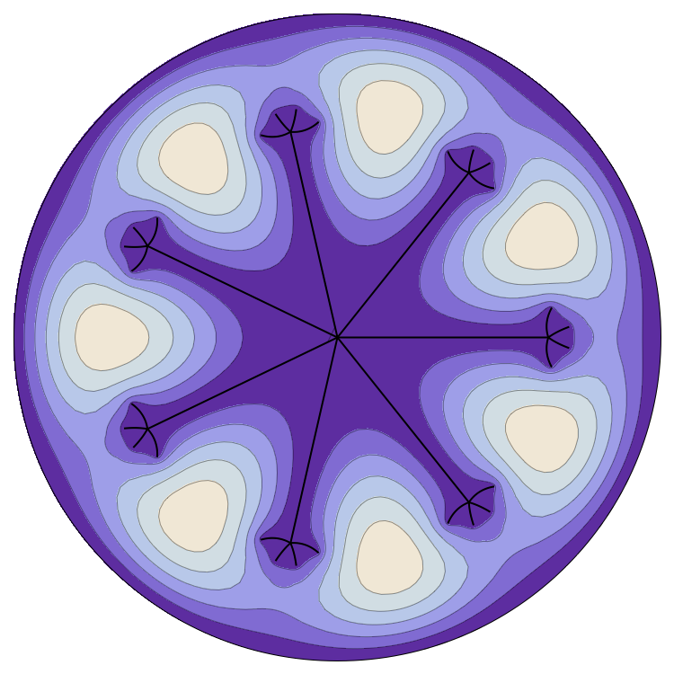
The strongest singularity, \(r^{\alpha}\), occurs for eigenvectors
associated with the first eigenvalue \(\lambda_1=\lambda_{1,1}\), and
its latter occurrences depend on how the roots of \(J_{\sigma_1}\) are
distributed in relation to those of \(J_{\sigma_k}\) for \(k\geq 1\).
For example, when \(\alpha=1/2\), the first several eigenvalues
are given below in a scatter plot, organized as follows: for each
\(m\) indicated on the x-axis, we see the eigenvalues
\([j_m(k/2)]^2\) for increasing \(k\) stacked above it. The
eigenvalues \([j_m(1/2)]^2=(m\pi)^2\) whose eigenvectors have an
\(r^{1/2}\)-singularity at the origin, are marked in red; and the
dashed lines help indicate how the gap between where these occur in
the spectrum increases.
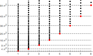
More specifically, the first eight occurrences of a
\(r^{1/2}\)-type singularity are associated with the eigenvalues:
\[
\begin{array}{ll}
\lambda_1=\lambda_{1,1}=\pi^2&\lambda_6=\lambda_{1,2}= 4\pi^2\\
\lambda_{17}=\lambda_{1,3}=9\pi^2&\lambda_{32}=\lambda_{1,4}= 16\pi^2\\
\lambda_{53}=\lambda_{1,5}=25\pi^2&\lambda_{76}=\lambda_{1,6}= 36\pi^2\\
\lambda_{107}=\lambda_{1,7}=49\pi^2&\lambda_{143}=\lambda_{1,8}= 64\pi^2
\end{array}
\]
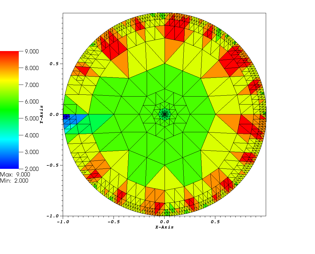
Employing a sequence of hp-adapted meshes obtained using the
Discontinuous Galerkin approach described in
- S. Giani and E. Hall. An A Posteriori Error Estimator for
hp-Adaptive Discontinuous Galerkin Methods for Elliptic Eigenvalue
Problems. Mathematical Models and Methods in Applied Sciences
(M3AS), 22(10):1250030, 2012.
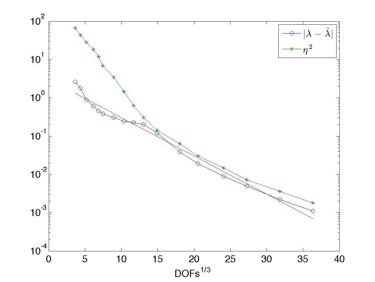
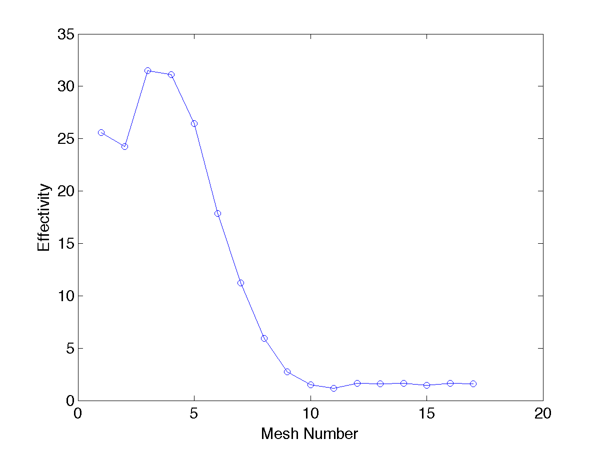
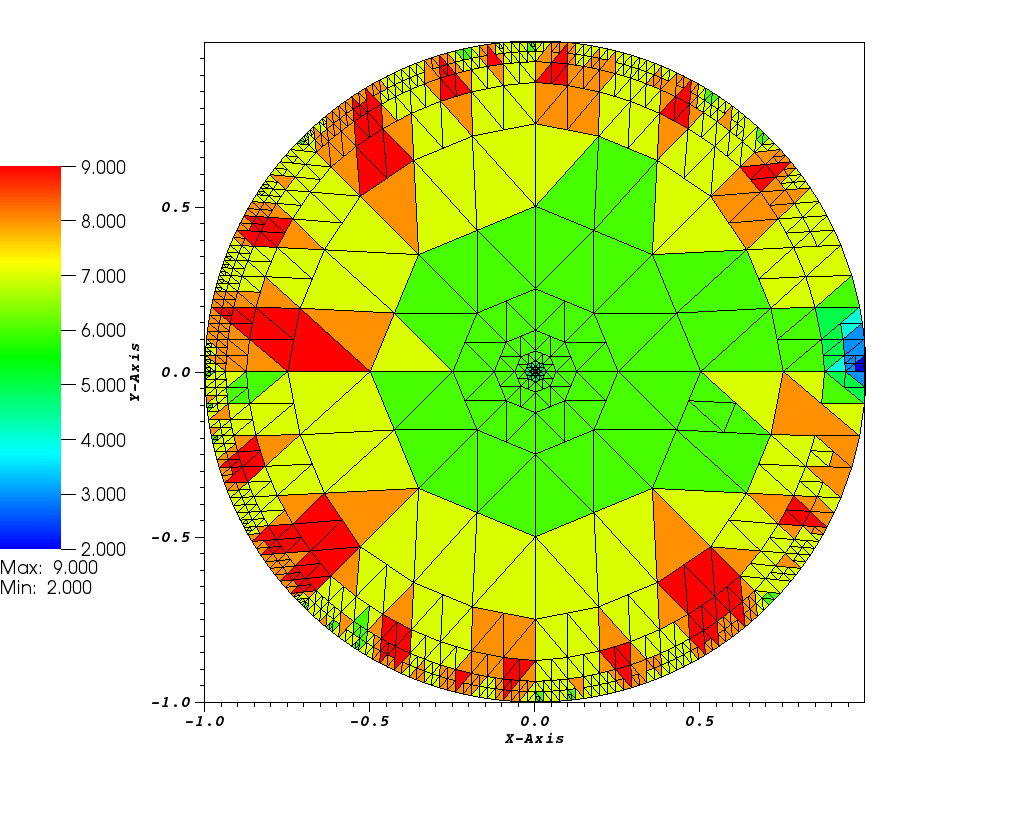
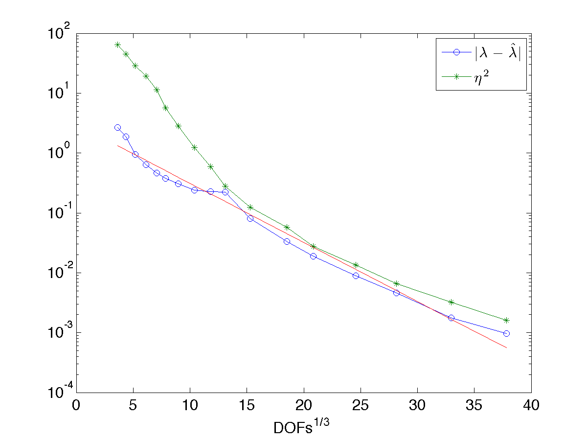
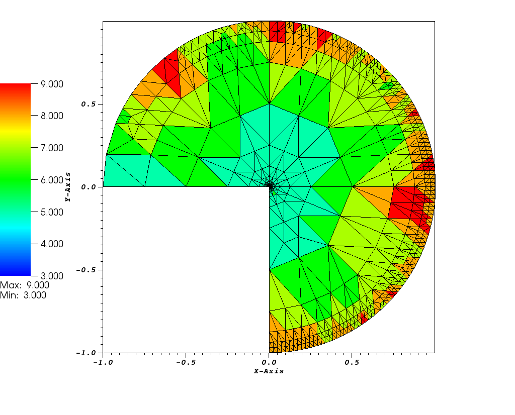
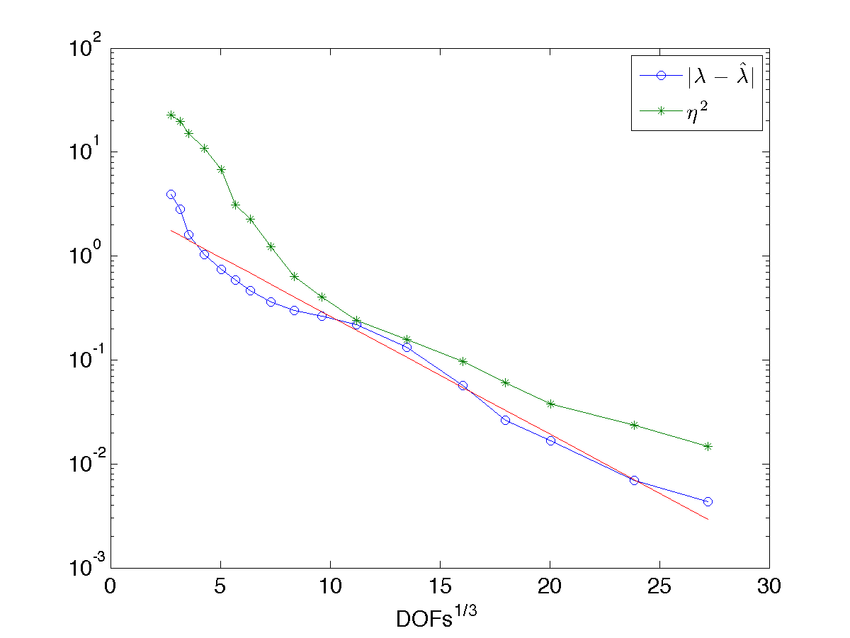
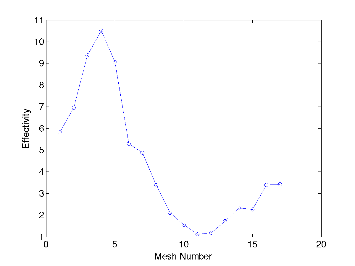
The final mesh (top) is given together with a history of the errors and
error estimates (lower left), and the corresponding effectivities (lower right),
EFF = (error
estimate)/(true error),
for the smallest eigenvalue when
\(\alpha=1/2\).
We note that this is not an indefinite problem, but the algorithm
described in the paper above can be applied.
Dirichlet condition on \(r=1\),
Neumann conditions on \(\theta=0\) and \(\theta=\alpha\pi\)
All eigenpairs doubly-indexed, \( (u_{km},\lambda_{km})\):
\[
u_{km}=J_{\sigma_k}(j_m(\sigma_k)\,r)\,\cos(\sigma_k\,\theta)\quad,\quad
\lambda_{km}=[j_m(\sigma_k)]^2\quad,\quad
\sigma_k=k\alpha\quad,\quad k\geq 0\;,\; m\geq 1
\]
Here, the eigenmode associated with the smallest eigenvalue
\(\lambda_1=\lambda_{0,1}\) are analytic, and the strongest
singularity, \(r^\alpha\), first occurs in eigenmodes associated with
the second eigenvalue, \(\lambda_2=\lambda_{1,1}\). For example, when
when \(\alpha=1/2\),
\(\lambda_1=\lambda_{0,1}\approx 5.78318596294678452117599575846\),
\(\lambda_2=\lambda_{1,1}=\pi^2\),
and
the next occurrence of
a \(r^{1/2}\)-type singularity is for the eigth eigenvalue
\(\lambda_8=\lambda_{1,2}=4\pi^2 \).
Dirichlet condition on \(r=1\),
Dirichlet condition on \(\theta=0\) and Neumann condition on \(\theta=\alpha\pi\)
All eigenpairs doubly-indexed, \( (u_{km},\lambda_{km})\):
\[
u_{km}=J_{\sigma_k}(j_m(\sigma_k)\,r)\,\sin(\sigma_k\,\theta)\quad,\quad
\lambda_{km}=[j_m(\sigma_k)]^2\quad,\quad
\sigma_k=\frac{(2k+1)\alpha}{2}\quad,\quad k\geq 0\;,\; m\geq 1
\]
As in the Dirichlet-Dirichlet case, the strongest singularity, which
is \(r^{\alpha/2}\) in this case, occurs in the eigenmode associated
with the smallest eigenvalue \(\lambda_1=\lambda_{0,1}\). For
\(\alpha=1/2\), the first two occurrences of the strongest
singularity, \(r^{1/4}\) happen for
\(\lambda_1=\lambda_{0,1}\approx 7.73333653346596686390263803337\)
and \(\lambda_6=\lambda_{0,2}\approx
34.8825215790904790430911907100\).
In contrast, when \(\alpha=2/3\), the first two occurrences of the strongest
singularity, \(r^{1/3}\) happen for
\(\lambda_1=\lambda_{0,1}\approx 8.42500692949919857451071877294 \)
and \(\lambda_5=\lambda_{0,2}\approx
36.3940370569496758450772289141\).
Employing a sequence of hp-adapted meshes obtained using the
Discontinuous Galerkin approach described in
- S. Giani and E. Hall. An A Posteriori Error Estimator for
hp-Adaptive Discontinuous Galerkin Methods for Elliptic Eigenvalue
Problems. Mathematical Models and Methods in Applied Sciences
(M3AS), 22(10):1250030, 2012.
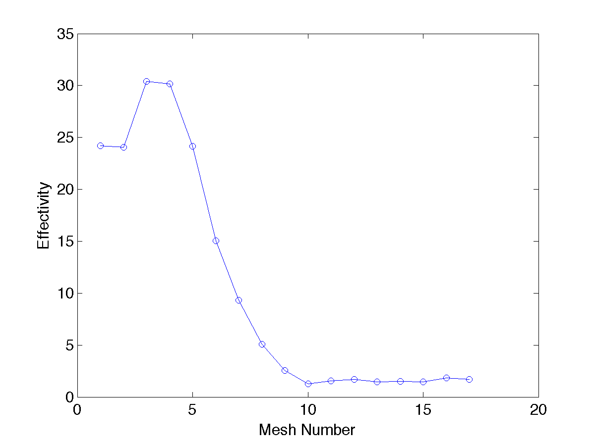
The final mesh (top) is given together with a history of the errors and
error estimates (lower left), and the corresponding effectivities (lower right),
EFF = (error
estimate)/(true error),
for the smallest eigenvalue when
\(\alpha=1/2\).
We note that this is not an indefinite problem, but the algorithm
described in the paper above can be applied.
The same experimental results are reported for the
"Pac-man" shape \(\alpha=2/3\), using instead the Continuous Galerkin
approach described in
- S. Giani, L. Grubišić, and J. Ovall. Error control for
hp-adaptive approximations of semi-definite eigenvalue
problems. Computing, 95(1):235–257, 2013.
which can certainly be applied to problems which are positive definite.